Distributed Logging: Metrics & Reports
Metrics
Low dimensionality, aggregation, monitoring and alerts. Inside of all metric collection systems are the time series databases. These databases do an excellent job of aggregation, so metrics are suitable for aggregation, monitoring, and building alerts.
For metrics, the dimension of the data should not exceed a thousand. If we add some Request IDs for which the size of the values is unlimited, then we will quickly encounter serious problems. We have already stepped on this problems.
Correlation and trace
Structured logs are not enough for us to conveniently search by data. There should be fields with certain values: Request ID, User ID, other data from the services from which the logs came.
The traditional solution is to assign a unique ID to the transaction (log) at the entrance to the system. Then this ID (context) is forwarded through the entire system through a chain of calls within a service or between services.
There are well-established terms. The trace is split into spans and shows the call stack of one service relative to another, one method relative to another relative to the timeline. You can clearly trace the message path, all timings.
First we used Zipkin. Already in 2015, we had a Proof of Concept (pilot project) of these solutions.
To make everything correct, the code needs to be instrumented. If you are already working with a code base that exists, you need to go through it – it requires changes.
For a complete picture and to benefit from the traces, you need to instrument all the services in the chain, and not just one service that you are currently working on.
This is a powerful tool, but it requires significant administration and hardware costs, so we switched from Zipkin to another solution that is provided “as a service”.
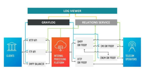
Delivery Reports
Logs must be correlated. Traces must also be correlated. We need a single ID – a common context that can be forwarded throughout the call chain. But often this is not possible – correlation occurs within the system as a result of its operation. When we start one or more transactions, we still do not know that they are part of a single large whole.
Lets consider the first example.
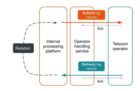
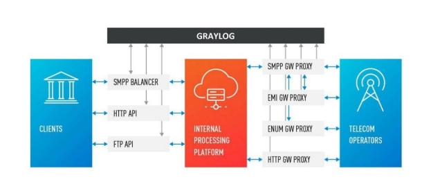
The client sent a request for a message, and our internal platform processed it.
The service, which is engaged in interaction with the operator, sent this message to the operator – an entry appeared in the log system.
Later, the operator sends us a delivery report.
The processing service does not know which message this delivery report relates to. This relationship is created later in our platform.
Two related transactions are parts of a single whole transaction. This information is very important for support engineers and integration developers. But this is completely impossible to see based on a single trace or a single ID.
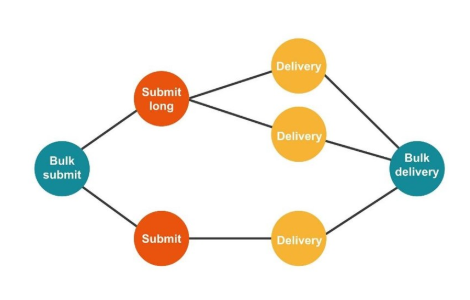
The second case is similar – the client sends us a message in a large bundle, then we disassemble them, they also return in packs. The number of packs may even vary, but then all of them are combined.
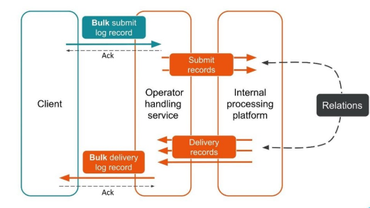
From the point of view of the client, he sent a message and received a response. But we got several independent transactions that need to be combined. It turns out a one-to-many relationship, and with a delivery report – one to one. This is essentially a graph.
Neo4j
We implemented Proof of Concept: a 16-core host that could process a graph of 100 million nodes and 150 million links. The graph occupied only 15 GB of disk – then it suited us.
In addition to Neo4j, we now have a simple interface for viewing related logs. With him, the engineers see the whole picture.
But pretty quickly, we became disappointed in this database.
Problems with Neo4j
Data rotation. We have powerful volumes and data must be rotated. But when deleting a node from Neo4j, data on the disk is not cleared. I had to build a complex solution and completely rebuild the graphs.
Performance. All graph databases are read-only. On recording, performance is noticeably less. Our case is absolutely the opposite: we write a lot and relatively rarely read – these are units of requests per second or even per minute.
High availability and cluster analysis for a fee. On our scale, this tranformes into decent costs.
Therefore, we went the other way.
Solution with PostgreSQL
We decided that since we rarely read, the graph can be built on spot when reading. So we in the PostgreSQL relational database store the adjacency list of our IDs in the form of a simple table with two columns and an index on both. When the request arrives, we bypass the connectivity graph using the familiar DFS algorithm (depth traversal), and get all the associated IDs. But this is necessary.
Data rotation is also easy to solve. For each day we start a new table and after a few days, when the time comes, we delete it and release the data. A simple solution.
We now have 850 million connections in PostgreSQL, they occupy 100 GB of disk. We write there at a speed of 30 thousand per second, and for this in the database there are only two VMs with 2 CPUs and 6 GB RAM. As required, PostgreSQL can write longs quickly.
There are still small machines for the service itself, which rotate and control.
